The New Feudalism: Why States Must Repeal Growth‐​Management Laws

Median home prices in growth-managed regions are typically two to four times more than those in unmanaged areas. Growth restrictions also dramatically increase home price volatility, making homeownership a riskier investment. Growth management slows regional growth, exacerbates income inequality, and particularly harms low-income families, especially minorities such as African Americans and Latinos.

By Randal O’Toole

Growth-management laws and plans, which strictly regulate what people can and cannot do with their land in the name of controlling urban sprawl, do far more harm than good and should be repealed.

To correct the problems created by growth management, states should restrict the authority of municipal governments, especially counties, to regulate land uses. Some 13 states have growth-management laws that require local governments to attempt to contain urban growth. These laws take development rights from rural landowners and effectively create a “new feudalism” in which the government decides who gets to develop their land and how. The strictest laws are in California and Hawaii, followed by Oregon, Washington, New Jersey, and several Northeastern states.

Growth-management advocates say that their policies protect farms and open space, save energy and reduce air pollution, and reduce urban service costs. However, farms and open space hardly need saving, as the nation has an abundance of both. There are much better ways of saving energy and reducing pollution that cost less and don’t make housing unaffordable. Finally, the costs of growth management are far greater than the costs of letting people live in densities that they prefer.

As compared to the trivial or nonexistent benefits of growth management, the costs are huge. Median home prices in growth-managed regions are typically two to four times more than those in unmanaged areas. Growth restrictions also dramatically increase home price volatility, making homeownership a riskier investment. Growth management slows regional growth, exacerbates income inequality, and particularly harms low-income families, especially minorities such as African Americans and Latinos.

The key to keeping housing affordable is exactly the opposite of what growth management prescribes: minimizing the regulation of vacant lands outside of incorporated cities. Allowing developers to build on those lands in response to market demand will also discourage cities from overregulation lest they unnecessarily push development outside the city

Introduction

Under the feudalistic system of medieval Europe the monarch owned all of the land in a country and people were allowed to use that land only at his or her sufferance and by paying an annual royalty to the monarch. Substitute “government” for “monarch” and this system still prevails in most of the world today, including much of Africa, Asia, and South America.

In the “more enlightened” parts of Europe and North America, however, a new kind of feudalism has taken hold. Under this new feudalism people may own private property, but what they can do with that property is strictly controlled by the government. The new feudalism was pioneered by Great Britain in 1947, but has since been adopted by many other European countries, Australia, New Zealand, and by several American states and Canadian provinces, most notably British Columbia, California, Florida, Hawaii, Oregon, Washington, and several Northeastern states.

The policies that restrict private property under the new feudalism are collectively known to urban planners as growth management.¹ These include any policies designed to influence either where or how fast growth takes place. The most popular form of growth management today is smart growth, which focuses on limiting the expansion of urban areas and increasing population densities in areas that are already urbanized. Some older forms of growth management, which might be called slow growth, attempted to limit the expansion of urban areas while also limiting the density or growth rates of those areas.

Advocates of growth management say that it produces many benefits, including preservation of farm lands, energy savings, reduced air pollution, and lower infrastructure costs. In fact, these benefits are either imaginary or could more easily be achieved in other ways without restricting property rights.

Farm lands, for example, are extremely abundant and do not need protection from urbanization. More energy can be saved and pollution reduced at a far lower cost by making motor vehicles and buildings more energy efficient than by attempting to influence land-use patterns. The small savings in infrastructure costs from growth management also pale in comparison to the high costs of growth management.

In comparison with the dubious benefits of growth management, the costs are overwhelming. The most quantifiable cost is the effect on housing prices. Housing typically costs two to five times more in states with growth-management laws than in states without such laws. While the data are not as readily available for commercial and industrial real estate, growth management has similar effects on their prices as well.

Growth management also increases the volatility of real estate prices, leading to bubbles. In places with no growth management, real estate bubbles are so rare as to be nearly nonexistent. But most places that pass growth-management laws soon begin to experience volatile prices and bubbles: Britain has had at least three bubbles since passing its 1947 law; California has had three and is entering a fourth; and Oregon has had two and is entering a third. Increased volatility discourages homeownership by increasing the risk of purchasing a home.

By increasing real estate prices, growth management slows the growth of states and regions that have adopted it and, in turn, of the nation as a whole. While many states that have not adopted growth management have grown faster as a result of people and businesses migrating from growth-managed states, the cost of such migrations are a deadweight loss on society. As a result, the nation’s overall growth in gross domestic product is close to 10 percent lower than it would be without growth management.

Another major cost is an increase in income and wealth inequality. Indeed, much of the increase in inequality since 1968 (when American inequality was at its lowest) is due to growth management enriching existing homeowners while impoverishing new home buyers and renters.

A final major cost is unemployment. Normally, homeowners have lower unemployment rates than renters. But growth management reverses this because it can make selling a house and moving crushingly expensive. Thus, many homeowners in growth-managed regions remain unemployed rather than search for work in other parts of the country.

These costs fall disproportionately on low-income families, many of whom are minorities. The effect of growth management can be seen by considering African Americans, who remain the least economically mobile minority in America. While urban areas with the most intensive growth management, such as the San Francisco Bay Area and Honolulu, continue to grow, albeit slowly, their Black populations are often declining. African American populations in other growth-managed areas may be growing, but the quality of the housing they live in is declining.

For all these reasons, it is imperative that states repeal laws mandating or authorizing city, county, and regional governments to practice growth management. Local and regional governments that practice growth management should abolish their plans.

The History of Growth Management

The first democratic nation to use growth management was the United Kingdom, whose parliament passed the Town & Country Planning Act in 1947. This law established large greenbelts around all major cities and forbade new developments in those belts.² Later laws restricted development on most other rural lands as well. A small number of people own most rural land in Britain: just 36,000 own half the land in the country.³ Those landowners were compensated with an annual payment that today exceeds $120 per acre, or more than $5 billion per year nationwide.⁴ Britain’s example inspired many European nations, as well as Australia and New Zealand, to pass similar laws, while in Canada, the British Columbia legislature passed the first of several increasingly restrictive laws, beginning with the Town Planning Act in 1949, and most recently, the Growth Strategies Act of 1995.⁵

In 1961, Hawaii became the first American state to pass a growth-management law. Act 187 divided the state into three types of land: urban, agriculture, and conservation, and restricted development on the latter two types. In 1963, a fourth type was added, rural, probably to keep undeveloped lands from being urbanized even if they had no agricultural or conservation value.⁶

In 1963, the California legislature passed AB 1662, sometimes called the Knox-Nesbit Act, to regulate city annexations and the formation of new cities and service districts.⁷ Although not intended to be a growth-management law, AB 1662 placed authority over annexations and new governments in the hands of the cities. The cities soon realized that they could force most new development (and associated tax revenues) to stay within their borders by denying applications for new cities and service districts. Many cities and counties soon drew urban-growth boundaries outside of which development was strictly limited.

The barriers to growth created by this law were compounded by the 1970 passage of the California Environmental Quality Act, which required a detailed analysis prior to any public actions. State courts held that expanding an urban-growth boundary required such an analysis, the cost of which became so prohibitive that boundaries are almost never expanded.

The Los Angeles, San Diego, and San Francisco-Oakland urban areas are all heavily constrained by these laws. For example, only 34 percent of the five counties in which the San Francisco-Oakland urban area is located have been urbanized. About 20 percent is public land, leaving 45 percent available for urbanization. But this land, although it is private, cannot be developed because of growth boundaries and other government restrictions. Similarly, two-thirds of the three-county Los Angeles area (Los Angeles, Orange, and Ventura counties) and more than 80 percent of San Diego County are undeveloped rural land.⁸

Taken together, California’s laws could be considered a slow-growth-management scheme rather than smart growth, as many of the cities and counties that passed urban-growth boundaries also limited population densities within the boundaries. In 2008, the California legislature attempted to convert this to smart growth by passing Senate Bill 375, which requires cities to rezone to higher densities, supposedly in order to reduce greenhouse gas emissions.⁹ Yet the densities of major California urban areas had already increased to well above the national average for urbanized areas of about 2,500 people per square mile. Between 1980 and 2010, San Francisco’s urban density grew by 32 percent to 5,300 people per square mile; Los Angeles’ by 28 percent to 6,620 people per square mile; and San Diego’s by 45 percent to 4,040 people per square mile.¹⁰

Between 1970 and 2000, 11 more states passed statewide planning laws, most of which ended up requiring urban-growth boundaries around most or all cities in those states: Vermont (1970), Oregon (1973), Connecticut (1974), Florida (1985), New Hampshire (1985), New Jersey (1986), Maine (1988), Rhode Island (1988), Washington (1990), Maryland (1992), and Delaware (1995).¹¹ Georgia passed a state planning law in 1989 but never implemented growth boundaries.¹² Tennessee passed a 1998 planning law that requires urban-growth boundaries, but those boundaries are solely used to determine where cities may annex land, not to manage growth. Florida partially repealed its law in 2011.¹³

Of the states that mandate urban-growth boundaries, Oregon’s law is typical and has served as the model for many of the other states. Oregon’s Senate Bill 100 created a state land-use commission that wrote rules that cities and counties were required to follow in their planning and zoning. The commission required that every city have a growth boundary. Although the law requires cities to expand boundaries to meet future housing needs, a 1993 amendment allows them to meet those needs by rezoning neighborhoods within the boundaries to higher densities.

A few other states do not have explicit growth-management laws but still have effective limits on growth. Nearly 85 percent of Nevada is owned by the federal government, and this has hampered growth in the Las Vegas and Reno urban areas. Like most New England states, Massachusetts has mostly given up on the county level of government, so cities and townships control land uses and have limited the geographic expansion of Boston and other cities.

A few cities and urban areas outside of these states also practice growth management. Most notable is Boulder, Colorado, which has purchased land or easements to form a greenbelt around the city equal to more than nine times the land area of the city itself. Boulder’s plan was a slow-growth plan, as it also limited the number of building permits that could be issued within the city each year. The Denver and Minneapolis-St. Paul urban areas also have urban-growth or urban-service boundaries outside of which new development is restricted.

Loudoun County, in northern Virginia, uses large-lot zoning to discourage new development, while Montgomery County, Maryland, has placed most of the undeveloped land in the county in either an agricultural reserve or in easements. Together, these limit the growth of the Washington, D.C., urban area.

Most other cities in America have zoning, but zoning is not growth management. In most cases, zoning exists to protect existing neighborhoods from unwanted intrusions, and many cities and counties readily change zoning at the request of landowners when the changes will not significantly affect neighbors.

Texas does not authorize counties to zone. This allows developers to maintain a large supply of buildable lots that can absorb the rapid population growth of Dallas-Ft. Worth, Houston, San Antonio, and other Texas urban areas. Other states, including Indiana and Nevada, allow counties to zone but do not require it, and several counties in these states don’t zone. Even where counties do zone, they tend to be highly flexible, often putting undeveloped land in a “holding zone” that they will happily alter if the landowners want to develop the property.

Zoning is far from perfect, but city zoning alone does not make housing unaffordable. What makes housing unaffordable is restrictions on development outside the cities. So long as a significant inventory of land is available for development outside of a city, the region will have room to grow and the city itself will have an incentive to minimize land-use regulation lest it lose new developments — and the resulting tax revenues — to the county or other nearby cities. Growth management, whether slow growth or smart growth, aims to use state and regional governments to restrict rural development in order to force most growth into the cities. The cities, in turn, then impose even more restrictions because they know that developers have nowhere else to go.

In sum, growth management affects housing markets in about a dozen states and several more urban areas. It also affects housing markets in cities adjacent to those states. Since Connecticut and New Jersey both have growth management, New York City is affected. Since Maryland and northern Virginia counties both have growth management, Washington, D.C., is affected. In total, around 40 percent of all American housing is made artificially expensive by growth management.

The Benefits of Growth Management

Advocates of growth management argue that it will do everything from curing obesity to reducing teenage angst. Most of these claims are absurd.¹⁴ However, at least three arguments deserve detailed consideration as they are most often cited and fervently believed by many public officials. Growth management is necessary, they say, to preserve farms, forests, and open space; to save energy and reduce pollution; and to minimize the costs of infrastructure and urban services.

Saving Farms, Forests, and Open Spaces

The supposed need to protect farms, forests, and open space from urban sprawl is probably the most cited reason for growth management. Yet America is a big country and urbanization is no threat to the nation’s abundance of green spaces. Creating artificial shortages of housing and other urban land uses in order to protect lands that are abundant is poor policy.

The U.S. Department of Agriculture says that, as of 2012, the 48 contiguous states have more than 900 million acres of agricultural land, of which only about 362 million acres (40 percent) is used for growing crops.¹⁵ Moreover, the number of acres needed for growing crops has shrunk from 421 million acres in 1982 because per-acre yields of most major crops have grown faster than our population.¹⁶ As a result, says the department, urbanization “is not considered a threat to the Nation’s food production.”¹⁷

Forests are also abundant. The Forest Service says that the United States had 766 million acres of forests in 2012, up from 721 million acres in 1920.¹⁸ The increase is mostly due to the automobile and other motor-powered vehicles that replaced horses and other animal power and allowed farmers to convert tens of millions of acres of pasture land to croplands and forests. Timber inventories have grown from 616 million cubic feet of wood in 1953 to 972 million cubic feet in 2012 because forests have been growing and continue to grow considerably faster than they have been cut.¹⁹

Finally, open space is the most abundant land we have, as it includes agricultural lands, forests, and other green spaces. The Census Bureau says that, as of 2010, only 107 million acres of land have been urbanized in the contiguous 48 states, or just 3.6 percent of nearly 3 billion acres. The most heavily developed state, New Jersey, is still 60 percent rural open space.²⁰ Using a somewhat different definition of “urbanized,” the Department of Agriculture found 91 million acres were urbanized in 2012.²¹ Using either figure, more than 96 percent of the United States remains as rural open space.

There is little danger that population growth will render American farms, forests, and open spaces endangered in the future. The population of Britain is eight times denser than that of the United States, yet even that country has a surplus of rural lands. As economists with the London School of Economics observe, “planning policies seem to considerably overvalue the wider environmental and welfare costs arising from greenfield as compared to brownfield development and especially overvalue the prevention of development on all Greenbelt land regardless of that land’s actual environmental or amenity value.”²²

Saving Energy and Reducing Pollution

The claim that denser development will save energy by reducing the distances people need to drive was made in a 1973 book, Compact City, and has been an article of faith among urban planners ever since.²³ In fact, as explained in detail in a previous Cato policy analysis, The Myth of the Compact City, the data fail to support this idea.²⁴

As noted in that paper, the Transportation Research Board asked David Brownstone, an economist with the University of California-Irvine, to study this issue. After a detailed literature review, Brownstone found that most of the studies that found a major link between urban form and energy use were guilty of self-selection bias — that is, their finding that people living in dense neighborhoods drove less than those living in less-dense neighborhoods was due to the fact that people who didn’t want to drive tended to live in denser neighborhoods. Based on those studies that corrected for self-selection, Brownstone concluded that the link between density and driving was “too small to be useful” in saving energy or reducing pollution or greenhouse gas emissions.²⁵

To the extent that there is any link at all between density and environmental issues, there are far better ways to save energy and reduce emissions that cost less and do not require people to make major changes in lifestyles. For example, single-family “zero-energy” homes can be built for $125 per square foot, whereas high-rise housing typically costs well over $150 per square foot.²⁶ Similarly, cars can be made more energy efficient than they are today by substituting aluminum for steel, diesel engines for gasoline, and streamlining for boxy styles, all at a far lower cost than trying to shift people out of their cars and onto expensive transit systems.²⁷

Minimizing Infrastructure and Urban Service Costs

The third major justification for growth management is that it reduces the costs of infrastructure and urban services. A city that is twice as dense as another doesn’t need as many miles of streets, water and sewer pipes, and other infrastructure lines. This seems so obvious that urban planners rarely bother to test it.

As it turns out, it isn’t necessarily true that denser cities have lower infrastructure costs, or if it is, that reduction is small. A study by Duke University researcher Helen Ladd compared urban service costs with population densities. As urban planners would predict, Ladd found that urban service costs declined as densities increased up to a density of 200 people per square mile. However, at higher densities, urban service costs increased with increasing densities.²⁸ For reference, the Census Bureau defines densities greater than 1,000 people per square mile as urban and densities below that as rural, meaning that any urban density growth management could actually lead to higher urban service costs.

In 2004, Ladd’s work was updated by demographer Wendell Cox and economist Joshua Utt. They found that higher municipal densities were associated with slightly lower municipal costs per capita. Specifically, “each 1,000 increase in population per square mile is associated with a $43 per capita reduction in municipal expenditures.” In other words, “a virtually unprecedented increase in population density in an already urbanized area would trigger a decrease in expenditure equal to the price of dinner for two at a moderately priced restaurant.”²⁹

A study by urban planners at Rutgers University compared the costs of urban services for greenfield developments of different densities. The study concluded that higher density developments save about $11,000 per home.³⁰ Much, if not most, of this cost is paid by residents, so it is their choice whether to pay a little higher cost or live in higher densities. As will be shown in the next section, a cost of sprawl equal to $11,000 per home is a pittance compared with the cost of growth management.

The problem with the Rutgers costs-of-sprawl study is that, in most cases, the choice offered by growth-management planners is not to build greenfield developments at lower or higher densities but whether to build greenfield developments or to redevelop existing neighborhoods at higher densities. Portland, Oregon, for example, is attempting to meet nearly all future housing needs by such redevelopment. Yet it may cost much more to install infrastructure capable of supporting higher densities into existing areas than to develop greenfields. As urban researchers at Massachusetts Institute of Technology observed, “the cost of creating an additional unit of sewage or water-carrying capacity may be much higher than the unit cost of existing capacity if the old sewage or water lines must be dug up and replaced with larger ones.”³¹

Rather than attempt to control urban service costs by managing growth, municipal governments should work to ensure that people pay the costs of the services they use. Then people will be able to choose the densities they prefer to live in with a full understanding of the costs of their choices.

The Costs of Growth Management

Compared with the small and sometimes imaginary costs of sprawl, the costs of growth management are huge and reverberate throughout the entire economy. These costs include increases in land, housing, and other real estate prices; increased real estate volatility; a resulting reduction in economic productivity; growing wealth inequality; and increased unemployment.

Housing and Real Estate Prices

The most visible effect of growth management is a dramatic increase in housing prices and concurrent decline in housing affordability. Table 1 compares housing costs and affordability in 14 cities with growth management and 14 cities without growth management.

The first column of numbers shows the average price of a 2,200-square foot, four-bedroom, two-bath home in 2015 as calculated by the Coldwell-Banker home listing report.³² The second column shows the median price of a home as calculated by the 2014 American Community Survey (which means it is the median price in 2013).³³ The third column is a standard measure of housing affordability: the value-to-income ratio — that is, the median home value divided by median family income in that city in 2013.³⁴ Finally, the last column shows the population growth of the urban area in which the city is located for the years 2000 through 2010.³⁵

The 2,200-square-foot home price and median home price in most of the areas with growth management are both more than $400,000, while a similar 2,200-square-foot home costs between $200,000 and $300,000 and median prices are between $100,000 and $200,000 in most places without growth management. The few growth-managed cities with apparently low housing prices, such as Hartford and Providence, still have value-to-income ratios that are more than 4.0, while most cities without growth management have value-to-income ratios of 3.0 or less.

The more-affordable cities are not affordable because they are less desirable places to live. In fact, the growth column shows that most urban areas without growth management are growing much faster than most urban areas with it. Of course, affordable housing is a major reason why they are growing faster.

The cities listed in Table 1 are not exceptional. Table 2 shows that the states with the least-affordable housing tend to be those with a state growth-management act (shown in bold); states whose major cities are hemmed in by other states with growth management (for example, Washington, D.C., and New York City); or states whose major cities practice growth management without a state law (for example, Colorado, Montana, and Utah). Of states with growth-management laws, Maine is the most affordable, but at a value-to-income ratio of 2.82 it is still less affordable than the national average of 2.75.

Table 1. Housing Costs and Affordability

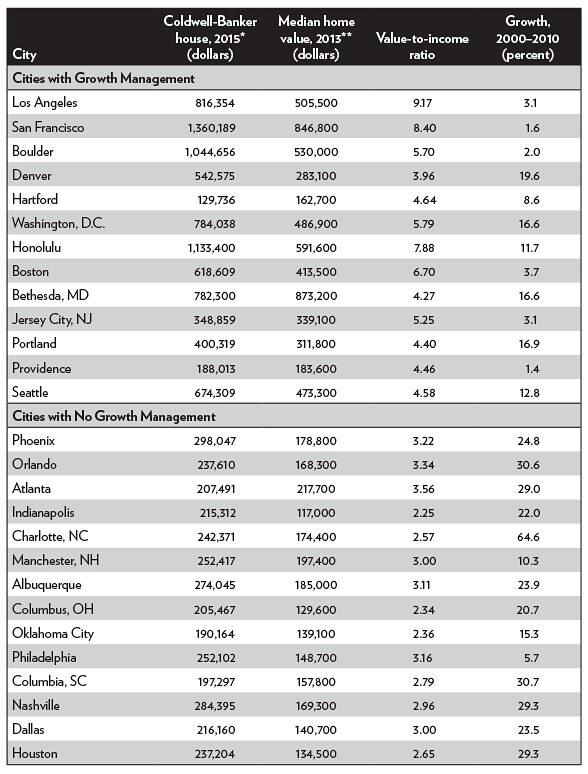
Sources: First column — Coldwell Banker, “2015 Home Listing Report,” 2015, tinyurl.com/CB2015HLR; second and third columns — 2014 American Community Survey, Census Bureau, 2015, median home values from table B25077 divided by median family incomes from table B19113 for places; fourth column — decennial censuses.

Notes: * The average price of a 2,200 square-foot four-bedroom, two-bath home as calculated by the Coldwell-Banker home listing report.

**Median price (half of homes are more expensive, half are less expensive) as calculated by the American Community Survey for the following year.

Table 2. State Housing Affordability

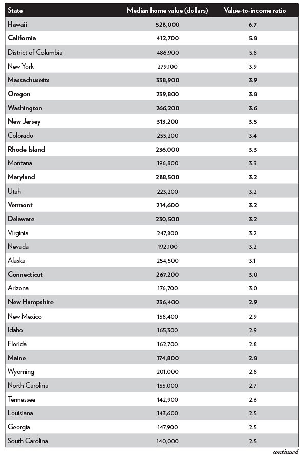
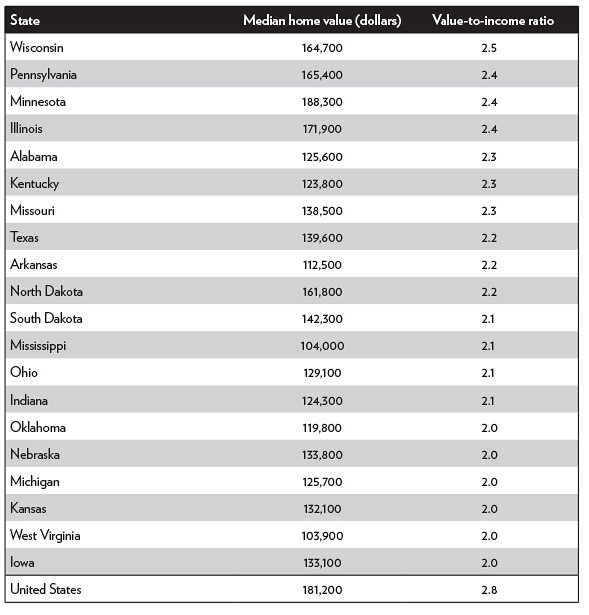
Source: 2014 American Community Survey, Census Bureau, 2015, median home values from table B25077 divided by median family incomes from table B19113 for places.

Note: Bold indicates states that have passed growth-management laws.

Housing is not the only real estate that is made less affordable by growth management. Industrial, commercial, retail, and other real estate also become more expensive. However, the best data we have are for housing, so housing should be read as a proxy for all real estate.

Urban planners often deny that growth management makes housing less affordable.³⁶ They seem to think that the laws of supply and demand don’t apply to residential land, so they can constrain the amount of land available for housing without making it expensive. But numerous studies by economists have reached the opposite conclusions. A few of these studies include:

• University of Washington economist Theo Eicher compared a database of land-use regulations with housing prices and found that high housing prices are “associated with cost-increasing land-use regulations (approval delays) and statewide growth management.”³⁷
• University of North Carolina real-estate economists Donald Jud and Daniel Winkler found that rapid growth in housing prices is strongly “correlated with restrictive growth management policies and limitations on land availability.”³⁸
• “Government regulation is responsible for high housing costs,” say Harvard economist Edward Glaeser and Wharton economist Joseph Gyourko.³⁹
• Canadian real-estate analysts Tsuriel Somerville and Christopher Mayer found that “Metropolitan areas with more extensive regulation can have up to 45 percent fewer [housing] starts and price elasticities that are more than 20 percent lower than those in less-regulated markets.”⁴⁰
• Federal Reserve economist Raven Malloy found that “in places with relatively few barriers to construction, an increase in housing demand leads to a large number of new housing units and only a moderate increase in housing prices,” while “places with more regulation experience a 17 percent smaller expansion of the housing stock and almost double the increase in housing prices.”⁴¹
• Research by economists Henry Pollakowsi and Susan Wachter concluded that “land-use regulations raise housing and developed land prices.”⁴²
• Three economists from the University of California-Berkeley found that “regulatory stringency is consistently associated with higher costs for construction, longer delays in completing projects, and greater uncertainty about the elapsed time to completion of residential developments.”⁴³

Home Price Volatility

Another predictable result of limiting the supply of land for housing is increased volatility. “Restricting housing supply leads to greater volatility in housing prices,” warns Glaeser.⁴⁴ In economic terms, growth management reduces the elasticity of the supply of land and housing. Supply price elasticity measures the response of supply to a change in demand; a low elasticity means the supply doesn’t respond as much, so small increases in demand can lead to large increases in price while small decreases in demand can lead to large decreases in price.

This is mentioned by Somerville and Mayer in their work and confirmed by other economists as well. “More restrictive residential land use regulations and geographic land constraints are linked to larger booms and busts in housing prices,” say economists Haifang Huang and Yao Tang. Their comparison of land-use regulations and housing prices in more than 300 cities in the United States found that, “the natural and man-made constraints also amplify price responses to an initial positive mortgage-credit supply shock, leading to greater price increases in the boom and subsequently bigger losses.”⁴⁵

Table 3 shows the volatility of value-to-income ratios by state for the years 1999 through 2013. Volatility is shown for value-to-income ratios rather than actual prices because prices partly reflect incomes and using value-to-income ratios accounts for changes in incomes over this time period. The first column of numbers shows the lowest value-to-income ratio during these years, the second shows the highest, while the third shows the value-to-income ratio in 2013. The last column shows the standard deviation of value-to-income ratios over this 15-year period as a measure of volatility.

Table 3. Volatility of State Value-to-Income Ratios, 1999-2013

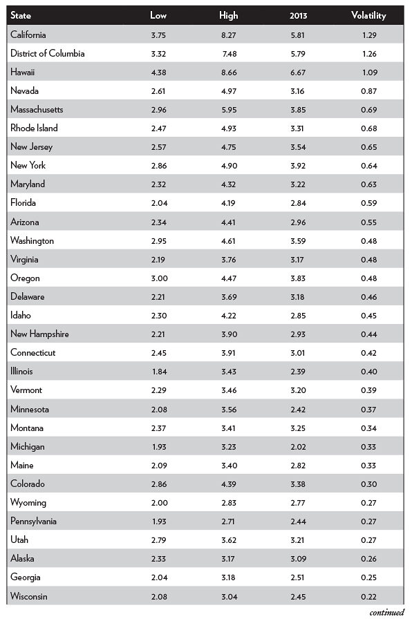
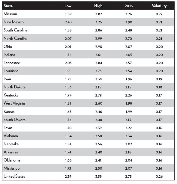
Source: Calculated from American Community Survey census data, tables P077 and H076 for 2000 through 2004 and tables B19113 and B25077 for 2005 through 2014. Census data present incomes and home values for the year before the survey was taken, so data from the 2014 American Community Survey is for 2013.

Note: The table includes the lowest and highest value-to-income ratios between 1999 and 2013, along with the 2013 value-to-income ratio and volatility, as represented by the standard deviation, over this time period.

Not surprisingly, the states with the strictest land-use laws, such as California and Hawaii, have the highest value-to-income ratios and volatilities. Volatilities are also high in the District of Columbia because of growth-management planning in counties surrounding D.C., just as they are high in New York City because of growth restrictions in the Connecticut and New Jersey counties that border the city. From California to Delaware, most of the 14 states with the most volatile housing prices have either state growth-management laws, strong local growth-management plans, or (in the case of Nevada and, to a lesser degree, Arizona) have urban growth limited by large amounts of state and federal land.

At the bottom end of the volatility scale are 18 states — South Carolina through Mississippi — that have minimal statewide planning laws and minimally restrictive local zoning codes. As noted above, most cities in these states use zoning as a way to protect existing development from unwanted intrusions, but they readily change the zoning of undeveloped lands to meet developer expectations of market demand. Not only does housing in these states have low volatility, but value-to-income ratios never reached 3.0.

In the middle are 18 states, from Idaho to New Mexico, with moderate volatilities and median housing values that sometimes exceeded three times median family incomes. In a few cases, such as Michigan and Wyoming, prices were volatile because of major changes in local industry (autos in Michigan, oil in Wyoming). A few other states, including Connecticut, Maine, and Vermont, have statewide planning laws that may not be quite as restrictive as the first 14 states on the list. But most of these states have one or more major urban areas that use some form of growth-management planning without a state mandate. Denver’s urban-growth boundary has already been mentioned; in Minnesota, the Twin Cities has an urban-service boundary; and several cities in Montana, including Kalispell, Missoula, and Bozeman, have worked with counties to restrict growth.

The increased volatility in housing prices that results from land-use restrictions greatly increases the risk in purchasing a home and is harmful in many other ways. Such volatility “transfers asset values between groups; creates financial instability. . . ; makes monetary policy more difficult . . . [and] create[s] oscillating wealth effects feeding through to consumption spending,” say economists from the London School of Economics.⁴⁶

Housing prices in growth-managed areas can undergo huge swings that are often called bubbles. The British housing market has experienced three bubbles since passage of the Town & Country Planning Act, peaking in 1973, 1989, and 2006.⁴⁷ California’s housing prices bubbled and peaked in 1981, 1990, and 2006. Oregon’s peaked in 1979 and 2006, while Massachusetts’s peaked in 1987 and 2006. Prices in growth-managed states are climbing rapidly today and in some regions, such as the San Francisco Bay Area, they have already exceeded the 2006 peak, suggesting that another crash is inevitable.

Notice that, prior to 2006, bubbles in local housing markets tended to offset one another, minimizing the effect on the nationwide housing market. This misled housing analysts in the early 2000s to believe that the bubbles that were then forming would not have major repercussions on the nation’s economy. Notably, Standard & Poor’s, Moody’s, and Fitch bond-rating companies gave many mortgage bonds AAA ratings because they did not imagine prices falling in so many markets at once. Banks that purchased such bonds were legally required to have a cash reserve equal to a fraction of the bond value that depended on the bond’s rating, with AAA bonds requiring reserves as little as 1.6 percent of a bond’s face value.

In 2007, ratings firms realized their mistake and began downgrading the bonds, sometimes reducing AAA mortgage bonds to lower than BBB ratings — that is, junk bonds. This increased the reserve requirements from 1.6 percent of the mortgage bond’s value to as much as 8 percent, which in turn forced banks such as Bear Stearns and Lehman Brothers to come up with hundreds of millions, or even billions, of dollars in cash overnight to meet the increased reserve requirement. Their inability to do so is what precipitated the 2008 financial crash.⁴⁸

While more bubbles may be on the horizon, the banks and bond ratings agencies have presumably learned their lesson and such a crash won’t happen again in this way. Still, it is fair to say that the 2008 crash can ultimately be traced to the volatility caused by growth-management planning, as without that volatility there would have been no bubbles and no need to downgrade mortgage bonds.

Regional Growth

High housing and real estate prices depress growth rates for two reasons. First, residents and investors are forced to put a higher share of their incomes into real estate, leaving less money to save or invest in more productive assets. Second, businesses are likely to move their operations to places with more affordable real estate.

The latter effect can be seen by comparing California and Texas. These are the nation’s first- and second-most populous states and the third- and second-largest states by land area. Both are located in the Sun Belt, and both are attractive to a wide range of industries, businesses, and people. But California’s land-use regulation has made it second only to Hawaii as the nation’s least-affordable housing market since the 1970s.

As a result, since 1990, Texas’s economic growth, measured in gross state product, has been 35 percent faster than California’s.⁴⁹ Since housing prices are a part of a state’s gross state product, California’s high housing prices mask some of the problems with the state’s economy. This is shown by Texas’s annual population growth, which has been 75 percent faster than California’s in the same time period.

While Texas benefits from California’s loss, the effects of high real estate prices on the national economy are not a zero-sum game. They are a negative-sum game, with real estate prices dragging down the economy in growth-managed regions more than other regions benefit. A paper by University of California-Berkeley economist Enrico Moretti and University of Chicago economist Chang-Tai Hsieh found that relieving land-use restrictions in productive cities such as New York and San Jose would increase the gross domestic product of the United States as a whole by 9.5 percent.⁵⁰ With a 2015 gross domestic product of $17.9 trillion, this represents an annual economic loss of $1.7 trillion.⁵¹

Unemployment

High and volatile housing prices can reduce labor mobility and increase unemployment rates by making it costly for people to move. In relatively unregulated housing markets, renters tend to have higher unemployment rates than homeowners. But Britain’s land-use regulation has turned this upside down, as homeowners are more likely to have higher unemployment rates.⁵² With real estate fees equal to a percentage of sale price, the cost of selling homes is a much higher share of people’s incomes: for example, if a family whose income is $50,000 sells a $100,000 home, a 5 percent realtor fee is 10 percent of their annual income. But if they sell a $500,000 home, a 5 percent fee is half their income. Add this to the higher down payment required for the more expensive home and the cost of moving can become prohibitive. Moreover, during economic downturns, homeowners in volatile housing markets are much more likely to owe more on a home than the house is currently worth. All of these things make it costly to move between or out of growth-managed areas.

Income Inequality

Income inequality has become a major issue in the United States and there is some reason for it, as the Gini index — which is used to measure income inequality — has grown since bottoming out in 1968.⁵³ According to Thomas Piketty in his book, Capital in the Twenty-First Century, income inequality is growing because returns on capital are greater than the rate of economic growth. But a refinement of Piketty’s work by MIT researcher Matthew Rognlie reveals that housing is the main source of growing inequality.

Looking closely at Piketty’s and other data, Rognlie found that “a single component of the capital stock — housing — accounts for nearly 100 percent of the long-term increase in the capital/income ratio, and more than 100 percent of the long-term increase in the net capital share of income.”⁵⁴ In other words, were it not for housing, inequality would not be growing. Moreover, the reason why housing capital stock is growing is that urban areas in most developed nations, including nearly every country in Europe, Australia, and many states, provinces, and major urban areas in the United States and Canada, have adopted policies intended to limit urban sprawl.

It may be no coincidence that American inequality reached its lowest level in 1968, before urban areas outside of Hawaii adopted growth-management plans.⁵⁵ American homeownership rates grew rapidly between 1940 and 1970, after which they leveled off. California and Oregon adopted growth-management planning in the early 1970s, leading homeownership rates in those cities to decline after that time. Today, homeownership nationwide stands at 63.5 percent.⁵⁶ But homeownership rates in some states without growth-management planning are nearly 75 percent.⁵⁷

The effect of growth management on homeownership is parallel to its effect on inequality. Harvard economists Peter Ganong and Daniel Shoag have shown that income inequality is growing in states where land-use restrictions have increased housing prices, while it continues to shrink (as it did before 1968) in states where there are few such restrictions. They conclude that “housing prices and building restrictions” played a “central role” in the growth of inequality since 1968.⁵⁸

Effect on Low-Income Groups

Low-income families are the hardest hit by growth management. Some urban areas have seen an outward migration of low- and, in a few cases, middle-income families because of high housing prices. As Glaeser writes, high housing prices will make a city “less diverse and instead evolve into a boutique city catering only to a small, highly educated elite.”⁵⁹ In other cases, low-income families have suffered a loss in housing quality, with declining homeownership rates and increasing shares living in multifamily housing.

African Americans are a useful bellwether, as their per capita incomes remain at about 60 percent of those of non-Hispanic Whites. Nationally, the number of African Americans grew by 11.0 percent between 2000 and 2010, while the overall population grew by 9.7 percent. But, as shown in Table 4, in many urban areas with growth management, the absolute number of Blacks fell or, at least, grew much more slowly than the overall population.

Among the nation’s 100 largest urbanized areas, the one with the greatest disparity between overall population growth and African American population growth was San Francisco-Oakland. Between 2000 and 2010, the overall population of this area grew by 9.5 percent, or 285,000 people, but the African American population shrank by 14.2 percent, or more than 48,000 people. Another region with a huge disparity is Los Angeles, whose urbanized area population grew by 3.1 percent, or more than 360,000 people, while the Black population declined by 11.4 percent, or nearly 106,000 people.

Other urban areas in which the overall population grew while the African American population declined include New York, Chicago, San Diego, San Jose, Tucson, and Honolulu. Two things most of these urban areas have in common are unaffordable housing and urban-growth boundaries or other land-use regulations restricting outward growth. By comparison, fast-growing regions that have minimal land-use restrictions, such as Atlanta, Dallas-Ft. Worth, and Houston, saw Black populations growing as fast, or faster, than overall populations.

In some urban areas with growth management, the number of African Americans did not decline, but the quality of housing they lived in did. In the Denver-Aurora urban area, for example, the share of families with White heads of households living in single-family housing declined slightly from 69.1 percent in 2000 to 67.8 percent in 2010. But the share of families with African American heads of households living in single-family housing dropped much more, from 54.0 to 46.4 percent.⁶⁰ Housing prices also affected tenure in the Denver-Aurora urbanized area: between 2000 and 2010, the share of Whites living in their own homes fell by 3.6 percent, but the share of African Americans (which was already well below the White share) fell by 11.9 percent.⁶¹

A 2015 Supreme Court decision held that any government policy that makes housing more expensive may potentially violate the Fair Housing Act. Even if a policy is not intentionally designed to discriminate against African Americans or other low-income minorities, if it has the effect of harming those minorities, then it is equally in violation of the law unless the policy can be “justified by a legitimate rationale.” This is known as the disparate impact doctrine.⁶²

Table 4. Change in Overall and African American Populations for Selected Urban Areas, 2000-2010

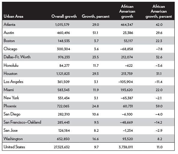
Source: 2000 Census, Table P003; 2010 Census, Table P1, for urbanized areas.

According to disparate-impact regulations published by the Department of Housing and Urban Development (HUD) in February 2013, conduct forbidden by the Fair Housing Act under this doctrine includes “enacting or implementing land-use rules, ordinances, policies, or procedures that restrict or deny housing opportunities or otherwise make unavailable or deny dwellings to persons because of race, color, religion, sex, handicap, familial status, or national origin.”⁶³ Numerous land-use rules, ordinances, and policies increase housing costs. Since some protected minorities, such as African Americans, are more likely to have lower-than-average incomes, any such rules or policies reduce their housing opportunities and therefore potentially violate the Fair Housing Act.

The HUD rules use two tests to determine whether a policy has a “legitimate rationale.” First, the legislative body or agency adopting the policy must show that it is “necessary to achieve one or more of its substantial, legitimate, nondiscriminatory interests.” Second is whether that interest “could be served by a practice that has a less discriminatory effect.”⁶⁴

For example, requiring that homes in urban areas be hooked up to sewage systems makes the houses a little more expensive but can be justified as a legitimate rationale based on public health concerns. However, saving farm land or open space is probably not a legitimate interest since the United States has an abundance of such land. Saving energy or reducing greenhouse gas emissions may be a legitimate interest, but there are other practices that can achieve these goals better and that do not have a discriminatory effect on low-income minorities. Thus, the disparate impact doctrine provides one more reason why states should repeal growth-management laws and regional and local governments should revoke growth-management plans.

Responses to Affordability Problems

Cities with serious housing affordability problems typically respond in one or both of two ways. First, many encourage developers to build denser housing, a policy that is informally known as build up, not out and more formally known as smart growth.⁶⁵ Second, they either subsidize or require that developers subsidize some housing for low-income buyers or renters, a policy known as affordable housing because it lowers the cost of a relatively few housing units, as distinct from housing affordability, which refers to the general level of housing prices relative to incomes.

The smart-growth strategy has been explicitly used in the Portland urban area at least since 1993. The region has focused on building higher-density housing since a law was passed that year that allowed Metro, Portland’s regional planning agency, to meet housing demand by directing local governments to rezone existing neighborhoods to higher densities. Partly as a result of this strategy, the population density of urbanized land in and around Portland has grown by 17 percent since 1990.

Until recently, the San Francisco Bay Area did not have a regional government powerful enough to force a smart-growth policy on cities in the region. Some cities actually adopted strict growth policies that, for example, forbade the construction of more than a few homes without a vote of the people. Despite this, the region’s population density increased even more than Portland’s, gaining 32 percent from 1980 to 2010 and 27 percent from 1990 to 2010.⁶⁶ Similarly, the density of the Los Angeles urbanized area grew by 28 percent between 1980 and 2010, while the Honolulu urbanized area grew by 9 percent and Seattle-Everett grew by 6 percent in the same time period.⁶⁷

These density increases, however, did not keep housing affordable. Between 1979 and 2009 the median value of homes relative to median family incomes grew by 37 percent in Portland, 76 percent in the San Francisco-Oakland area, 70 percent in Los Angeles, 19 percent in Honolulu, and 40 percent in Seattle-Everett.⁶⁸

In 2008, the California legislature passed SB 375, which directed regional governments such as the San Francisco Bay Metropolitan Transportation Commission (MTC) to write plans to increase population densities of cities in the region. The dual purpose of this increase was to reduce greenhouse gases and make housing more affordable. The MTC dutifully responded by writing Plan Bay Area. The plan calls for no expansion of urban-growth boundaries despite a projected 28 percent increase in population by the year 2040 and proposes to house this increase by targeting more than a quarter of the developed land in the region for redevelopment at higher densities. Yet the plan admits that this will fail to make housing more affordable, as the share of incomes that people are projected to spend on housing increases.⁶⁹

There are at least three reasons why rebuilding existing neighborhoods to higher densities will fail to make housing more affordable. First, construction of multifamily housing costs more per square foot than single-family housing. A study in Portland found that a multifamily dwelling typically costs 23 percent more per square foot than a single-family one. The study also found that high-rise housing costs per square foot were more than double the cost of two-story single-family construction.⁷⁰

Second, land costs in areas designated for high-density housing are often very high. While an acre of land suitable for single-family homes at the urban fringe might cost around $20,000, or $2,500 to $5,000 per developable lot, an acre of urban land designated for redevelopment to higher densities may cost hundreds of thousands or millions of dollars. Even if 50 units of housing are built on a single acre, the land cost per housing unit can be much more than for low-density greenfield developments.

Third, the cost of installing infrastructure in areas of existing development to support higher-density development is likely to be much higher than the cost of infrastructure in greenfield development. As noted above, so-called “cost of sprawl” studies compared the infrastructure costs of low-density greenfield development with high-density greenfield development, but not with high-density brownfield development. For all these reasons, high-density housing ends up being more affordable than low-density housing only if residents are willing to accept much smaller quarters in the high-density housing.

Census data confirm that higher densities are associated with less affordable housing. The 2010 Census reported population densities, median home values, and median family incomes for 382 urban areas and 558 cities. For urban areas, the correlation between affordability (measured by value-to-income ratios) and density is strong (correlation coefficient is 0.53), with a 1,000-person-per-square-mile increase in density being associated with an increase in value-to-income ratios of 0.64 (see Figure 1). For cities, the correlation is even stronger (correlation coefficient is 0.61), with the same population density increase being associated with an increase in value-to-income ratios of 0.27.⁷¹

Figure 1. Density and Housing Affordability

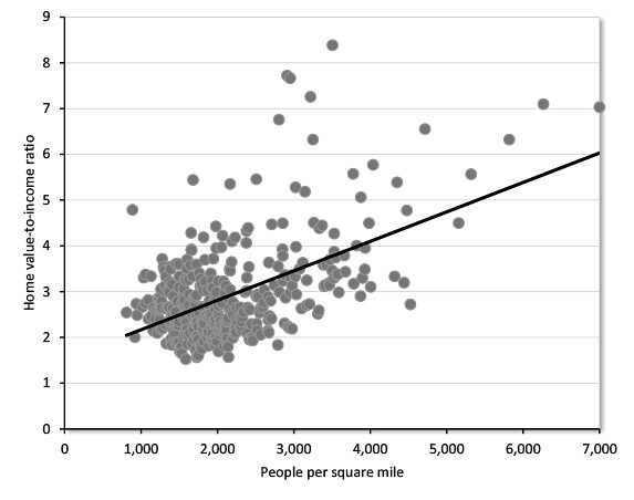
Note: The graph shows the average population densities and median home value to median family income ratios for 382 urbanized areas in the 2010 census.

Though density itself is not the sole direct cause of reduced housing affordability, the data show that factors associated with higher densities also tend to reduce affordability. Thus, the smart-growth strategy of building up, not out, will inevitably fail to maintain housing affordability.

The second local response to housing affordability problems is to subsidize the construction of selected units of housing and offer them to low-income buyers or renters at less-than-market prices — that is, the “affordable housing” policies mentioned above. Usually, sales of below-cost housing come with restrictions that buyers can only resell to other low-income people and only at the price they paid for it plus inflation. In effect, it turns owners of affordable homes into feudal peasants, allowed to sell their home only to people approved by the government at prices set by the government.

The bigger problem with affordable housing is that it confuses the problem of housing low-income people with the more general problem of housing affordability for everyone. Affordable housing programs such as subsidized housing and inclusionary zoning are aimed at providing a few units of housing for low-income people who might otherwise be homeless or be forced to live in housing that doesn’t meet some basic standards. These measures are completely ineffective against general housing affordability problems.

For example, median homes in Houston cost a little more than twice median family incomes, making it a fairly affordable region. Yet there still may be some people in Houston whose incomes are so low that they cannot afford decent housing. Affordable housing programs are aimed to help those people, and whether those programs work or are worthwhile is beyond the scope of this study.

In contrast, median homes in San Francisco cost more than eight times median family incomes, making it unaffordable to all but the wealthiest — and even they have to accept smaller or lower-quality homes than they might live in elsewhere. Affordable housing programs may help house a relative handful of people, but will not improve the overall level of affordability. While the government could theoretically swamp the market with affordable homes and thereby bring down the general price level, in reality the government doesn’t have the resources to build more than a tiny percentage of the homes being built in a region, so the effect of those affordable homes on the general price level is negligible.

Worse, some affordable housing policies actually make the remaining housing even less affordable. Some cities require homebuilders to sell or rent 15 to 25 percent of the homes they build to low-income families at below-market prices, a policy known as inclusionary zoning. Homebuilders respond by building fewer units of housing and by selling or renting the market-rate homes for higher prices to make up for their losses on the affordable homes. The result is that most renters and homebuyers end up paying more so that a relative handful can have affordable homes.⁷²

Other cities charge homebuilders a fee for every home they build and dedicate the revenues to the construction of affordable housing. For example, Portland recently imposed a 1 percent tax on the value of new homes. The funds raised by this tax over the next 30 years will be used to repay bonds needed to build 1,300 affordable homes.⁷³ Of course, the tax will raise the price of all housing in the city by 1 percent, while 1,300 new homes in a city that has more than 270,000 homes is not going to have a measurable impact on overall affordability.⁷⁴ Since anything that makes new homes more expensive also leads existing homeowners to increase the price of their homes when they sell them, overall housing affordability will decline.

Policies aimed at providing affordable housing for low-income people are not designed to deal with overall housing affordability. Affordable housing is a Band-Aid solution when the real solution is to end the policies that made housing unaffordable in the first place.

Growth Management vs. Exclusionary Zoning

Many fair-housing advocates blame housing affordability problems on exclusionary zoning, a form of zoning that, they say, is intended to make housing expensive so as to keep lower classes out of zoned neighborhoods, particularly in the suburbs. Without exclusionary zoning, they say, developers would respond to high-priced housing markets such as that in San Francisco by rebuilding existing neighborhoods to higher densities. These advocates usually ignore the role of urban-growth boundaries and other containment measures in local and regional housing markets. For example, a 30-page review of exclusionary zoning literature by legal scholar John Mangin never once mentions urban-growth boundaries.⁷⁵

When zoning was first developed in the early 20th century, some southern cities explicitly included racial requirements in their zoning codes. For example, Louisville’s first zoning code prohibited the sale of homes in some neighborhoods to African Americans. The Supreme Court ruled this unconstitutional in 1917.⁷⁶ Suburban communities then supposedly responded by writing their zoning codes to effectively require that homes be expensive, thus making housing unaffordable to low-income families.

The problem with this analysis is that zoning by itself does not make housing expensive or unaffordable. As Mangin notes, the basic cost of a home is “the cost of land plus construction costs and normal profit.”⁷⁷ As the Supreme Court noted in a 1926 decision, the purpose of zoning is to ensure that unwanted nuisances are not allowed to intrude into a neighborhood that would bring housing prices below this basic cost.⁷⁸ So long as there is competition for new home construction, zoning alone cannot raise the price of housing much above this basic cost. Amenities such as parks, good schools, and low crime rates may make particular neighborhoods more desirable, but these aren’t particularly influenced by zoning, and even if they were, better schools and less crime would have to be considered legitimate rationales for such policies.

It is only when competition for new home construction is limited — almost always by government regulation — that housing becomes more expensive than the basic cost of land plus construction. The smallest states have plenty of vacant land that can be used for home construction to maintain housing affordability. For example, New Jersey is the nation’s most heavily developed state, yet — as previously noted — 60 percent of the state remained undeveloped rural land as of 2012. Even the island of Oahu, Hawaii’s most crowded island, is 64 percent rural.⁷⁹ Without government restrictions on the use of such land, zoning cannot make housing much more expensive than its basic cost.

Zoning restrictions in some cities and suburbs may lead to income stratification in those communities. For example, some neighborhoods might be zoned for minimum lot sizes of one acre; other neighborhoods for one-half acre, one-quarter acre, or one-eighth of an acre. Some smaller incorporated suburbs may even zone all residential land in that suburb for larger lots, thus keeping out people who cannot afford that minimum lot size. In this sense, exclusionary zoning is real. Based on the disparate impact doctrine, it is potentially a violation of the Fair Housing Act if the city cannot find adequate justification for such zoning.

Some housing experts have recommended the use of regional governments to prevent this type of exclusionary zoning from taking place. For example, Glaeser suggests that “a more regional approach to housing supply might reduce the tendency of many localities to block new construction.”⁸⁰ However, an actual review of regional efforts to influence housing supply, such as those in Portland, Denver, and other urban areas that practice growth management, reveals that they do not produce this outcome; instead the political forces to limit housing supply overwhelm those aimed at promoting housing affordability.

For example, Oregon’s land-use planning system has set a goal of having “adequate numbers of needed housing units at price ranges and rent levels which are commensurate with the financial capabilities of Oregon households.” To meet this goal, all incorporated cities of 2,500 people or more have a full range of housing, including single-family and multifamily housing.⁸¹ Metro, the regional planning agency for Portland and 23 of its suburbs, interpreted this to mean that half of all new home construction in every city in the region must be multifamily housing, even though two-thirds of the region’s existing homes, and nearly all homes in some suburbs, are single-family housing.⁸²

This has put pressure on suburbs that are currently mostly single-family homes. When a multifamily subdivision in the suburb of Happy Valley failed, the landowners asked for a zoning change to allow single-family construction. Fair housing advocates charged that this violates Metro’s policy of requiring more compact development.⁸³

Yet there is no evidence that more multifamily housing would make the Portland area more affordable. As previously noted, multifamily housing costs more, per square foot, than single-family housing, so it is only more affordable if residents are willing to accept smaller homes.

Similarly, HUD has adopted regulations called “affirmatively furthering fair housing.” These rules require all governments that accept federal housing funds to assess whether they have a balance of incomes and races in their communities and, if not, to take steps to improve that balance.⁸⁴ In what many people see as a pioneering implementation of this rule, HUD ordered Westchester County, New York, to provide more low-income housing, mostly in the form of multifamily housing.⁸⁵

At heart, concerns over exclusionary zoning, and HUD’s response in the form of affirmatively furthering fair housing, have to do with racial segregation, not housing affordability. While stratification of neighborhoods by income may be a factor in racial segregation, forcing individual suburbs to build higher density housing is not likely to solve this problem. First, as noted, multifamily housing actually costs more per square foot than single-family. Second, without violating the Fair Housing Act, there is no way to ensure that people occupying supposedly affordable homes are racial minorities. Finally, HUD has a peculiar definition of “fair” if it thinks that minorities living in cramped apartments with little privacy is fair so long as those apartments are in the same suburbs as Whites who live in spacious single-family homes.

According to census data, residential segregation is declining throughout the nation.⁸⁶ As demographer William Frey says, as of the 2010 census, “minorities represent 35 percent of suburban residents, similar to their share of the overall U.S. population” and “more than half of all minority groups in large metro areas, including African Americans, now reside in the suburbs.”⁸⁷

However, segregation is declining in different communities for different reasons. In San Francisco, it is declining because housing prices have risen so high that many African Americans have been forced to leave the region entirely, leaving the region less segregated as Whites have replaced African Americans in neighborhoods that were formerly mostly Black. In Portland, it is declining because Whites are gentrifying traditional Black neighborhoods of rented single-family homes, forcing African Americans to move into multifamily housing in other parts of the region and making them more vulnerable to crime.⁸⁸ In Houston, segregation is declining because the region is rapidly growing, African American numbers are growing faster than Whites, and these African Americans are moving into neighborhoods throughout the region.

Evidence indicates that rapid population growth helps reduce segregation.⁸⁹ Policies that hinder that growth can severely harm minorities, as in the cases of San Francisco, where Black populations are shrinking, and Portland and Denver, where African Americans are forced into lower-quality housing.

The boundaries of incorporated suburbs tend to be based on historic factors that have far more to do with tax policies than racial politics. Many, if not most, suburbs incorporated to avoid being annexed and taxed by some nearby city. Because most suburbs represent only a small fraction of their urban area, they cannot be expected to all have a perfect balance of incomes and races. Rather than focus on the impossible goal of achieving such a perfect balance in each suburb, fair housing advocates should oppose the growth-management policies that make housing unaffordable in the first place.

Repealing Growth Management

The key to housing affordability is an unlimited supply of vacant land available for development at the urban fringe. “Unlimited” doesn’t mean “infinite”: it simply means that land isn’t limited by physical or legal limits on land development. A city on an island may have a physical limit to land development, but few American cities are on an island and those that are, such as Honolulu, still have plenty of undeveloped land available.

To restore housing affordability, reduce home price volatility, and remove barriers to local economic growth, states must repeal growth-management laws and take steps to forbid city and regional governments from practicing growth management or other regulations that limit the amount of vacant land available for development. This should be one of the highest legislative priorities in California, Florida, Hawaii, Maryland, New Jersey, Oregon, Virginia, and Washington, as well as in several New England states.

Florida partly repealed its growth-management law in 2011, but this appears to have failed to make housing more affordable because local governments kept their own stringent growth-control measures. The Florida story illustrates the need for serious, broad-reaching repeal of government growth management powers.

The state’s 1985 law required local governments to develop comprehensive plans aimed at preventing urban sprawl. Each plan had to be submitted to a state Department of Community Affairs for approval, and rejected plans had to be rewritten.

As early as 2001, Florida researchers found that “adoption of growth management regulations significantly raised home prices” and that growth management in general “reduces housing affordability for middle-class households.”⁹⁰ A more rapid decline in Florida housing affordability came after 1999: between 1999 and 2005, nominal median family incomes grew by 20 percent but median home values grew by 146 percent. This meant that housing costs, relative to family incomes, more than doubled.⁹¹

Alarmed about the effect of the law on housing prices, in 2011 the Florida legislature repealed the requirement that plans be approved by the Department of Community Affairs. However, local municipalities were still allowed to restrict development, and most continued to do so. Housing became far more affordable after the economic downturn, but after bottoming out in 2012, inflation-adjusted prices rose by more than 30 percent by the fourth quarter of 2014. This is in line with other growth-managed states — California prices rose 36 percent; Oregon’s 28 percent — which reduced housing affordability since 2011 as incomes did not keep pace with housing prices.⁹²

It is too early to tell for certain how the partial repeal of Florida’s growth-management law will affect housing affordability, but it appears that the effect will be minimal because cities and counties are maintaining their restrictions on greenfield development. Thus, more comprehensive reforms are needed to truly make housing affordable in growth-managed states and urban areas.

A more thorough reform would be for states to emulate Texas by restricting counties’ ability to zone or regulate land. Cities would still be free to zone to protect neighborhoods from nuisances, but the Dallas-Ft. Worth urban area shows that zoning alone isn’t a barrier to housing affordability. Cities in the Dallas-Ft. Worth urban area are zoned, yet the region’s population is growing nearly as fast as Houston’s, even though Houston and its largest suburb have no zoning. Dallas-Ft. Worth grew by 60 percent between 1990 and 2010, compared with Houston’s 70 percent, and the former remains just about as affordable, with a 2014 value-to-income ratio of 2.3, versus 2.2 in Houston.

An even more thorough reform, and one that could satisfy opponents of exclusionary zoning, would be for states to eliminate zoning altogether. If the purpose of zoning is to protect residential neighborhoods from the traffic, noise, pollution, and other problems that would result from intrusions of commercial, industrial, and higher-density residential uses, then that purpose is met in Houston (as well as on unincorporated lands in Texas) through the use of protective covenants.

About half of the neighborhoods in the city of Houston, and most in its suburbs, have such covenants. In most cases, covenants can be changed by a vote of 75 percent of a neighborhood’s residents. Neighborhoods that don’t have covenants can write them with the support of 75 percent of the residents. This system is flexible, affordable, and gives prospective residents a choice of neighborhoods that have a wide diversity of rules ranging from very strict to none at all.

Conclusion

Growth management takes away people’s property rights in the name of controlling urban sprawl, which is in fact a non-problem. Growth management results in huge transfers of wealth from renters and future homebuyers to people who owned homes at the time the growth-management rules were put into effect. It unnecessarily adds trillions of dollars to housing and other real estate costs even as it slows the economy by trillions of dollars a year.

The effects of growth management are greatest on low-income families, including many African Americans and Latinos. Regions with the most stringent growth-management rules have seen Black populations decline or be forced into lower-quality housing. Intentionally or not, growth-management plans effectively discriminate against working-class and poor families, large numbers of whom are racial minorities.

For all these reasons, the 13 states with state growth-management laws must repeal those laws and replace them with laws preventing counties from restricting development. Other states whose urban areas have written growth-management plans without a state mandate should also reduce the authority of counties to regulate land uses. These actions are the key to restoring housing affordability, reducing real estate volatility, and improving indicators of income inequality.

Notes

1. Arthur C. Nelson and James B. Duncan, Growth Management Principles and Practices (Chicago: American Planning Association, 1995), p. 1.
2. Peter Hall, Cities in Civilization (New York: Pantheon Books, 1998), p. 239.
3. Tamara Cohen, “Look Who Owns Britain,” Daily Mail (London), November 10, 2010, tinyurl.com/2wydny5.
4. Kevin Cahill, “The Great Property Swindle: Why Do So Few People in Britain Own So Much of Our Land?” New Statesman, March 11, 2011, tinyurl.com/4mr8cfk.
5. Randal O’Toole, Unlivable Strategies: The Greater Vancouver Regional District and the Livable Region Strategic Plan (Vancouver: Fraser Institute, 2007), p. 5.
6. Samuel B. K. Chang, “The Land Use Law Revisited: Land Uses Other Than Urban,” University of Hawaii, 1970, p. 2, tinyurl.com/jzg7mbw.
7. Paul Detwiler, “California within Limits: History of California’s Local Boundary Laws,” California Association of Local Area Formation Commissions, Sacramento, 2013, p. 8, tinyurl.com/hrq3794.
8. “Percent Urban and Rural in 2010 by State and County” (spreadsheet), Census Bureau, 2012, tinyurl.com/hu45vhd.
9. “The Basics of SB 375,” Institute for Local Government, Sacramento, 2015, tinyurl.com/79wlqxv.
10. 1980 Census of Population: United States Summary, Number of Inhabitants PC-80-1-A1 (Washington: Census Bureau, 1983), Table 34; and 2010 Census, Table G001, “Geographic Identifiers for Urbanized Areas.” To remain consistent with 1980 definitions of the San Francisco-Oakland and Los Angeles urbanized areas, data for the Concord and Livermore urbanized areas were included in the average for San Francisco-Oakland and data for the Mission Veijo and Santa Clarita urbanized areas were included in the average for Los Angeles in 2010.
11. Nichole Session Purcell, Statewide Planning and Growth Management Programs in the United States (Trenton: New Jersey Office of State Planning, 1997), p. iii, tinyurl.com/gwy7ftp.
12. Emily Ahlquist, Reggie Delahanty, Glenn Frankel, Ilan Guest, Liz Li, and Jing Xu, Smarten Up, Georgia! (Decatur, GA: Georgia Planning Association, 2007), p. 32, tinyurl.com/jazn8js.
13. Mary Ellen Klas, “Florida Lawmakers Wipe Out 30 Years of Growth Management Law,” Tampa Bay Times, May 7, 2011, tinyurl.com/jhednw7.
14. If they have any support at all, it comes from studies that confuse correlation with causation. For example, a study published by Smart Growth America claimed that urban sprawl causes obesity. (Barbara McCann and Reid Ewing, Measuring the Health Effects of Urban Sprawl (Washington: Smart Growth America, 2003), p. 1.) However, analyses by more objective researchers have found that, to the extent that there is a relationship between suburbs and obesity, it is because overweight people prefer to live in the suburbs, not that the suburbs made them overweight. (See, for example, Andrew J. Plantinga and Stephanie Bernell, “The Association between Urban Sprawl and Obesity: Is It a Two-Way Street?” Journal of Regional Science 47, no. 5 (2007): 857-79; and Jean Eid, Henry G. Overman, Diego Puga, and Matthew A. Turner, Fat City: Questioning the Relationship between Urban Sprawl and Obesity (Washington: Center for Economics and Policy Research, 2007), p. 1.
15. Summary Report, 2012 National Resources Inventory (Washington: Natural Resources Conservation Service, 2015), Table 2.
16. Crop Production Historical Track Records (Washington: Department of Agriculture, 2014).
17. Natural Resources Inventory: Highlights (Washington: Natural Resources Conservation Service, 2001), p. 1.
18. U.S. Forest Resource Facts and Trends (Washington: Forest Service, 2014), p. 8.
19. Ibid., p. 23.
20. “Percent Urban and Rural in 2010 by State and County”; 2012 National Resources Inventory, pp. 3-14.
21. 2012 National Resources Inventory, p. 3-2.
22. Paul C. Cheshire, Max Nathan, and Henry G. Overman, Urban Economics and Urban Policy: Challenging Conventional Policy Wisdom (Cheltenham, UK: Edward Elgar, 2014), p. 105.
23. George Dantzig and Thomas Saaty, Compact City: A Plan for a Livable Urban Environment (San Francisco: Freeman, 1973), p. 12.
24. Randal O’Toole, The Myth of the Compact City: Why Compact Development Is Not the Way to Reduce Carbon Dioxide Emissions, Cato Institute Policy Analysis no. 653, November 18, 2009.
25. David Brownstone, “Key Relationships between the Built Environment and VMT,” Transportation Research Board, 2008, p. 7, tinyurl.com/y9mro58.
26. Eric Thomas, “A Net-Zero-Energy House for $125 a Square Foot,” Green Building Advisor, January 7, 2013, tinyurl.com/jnhntyj; and Payton Chung, “Economics of Height,” West North, March 18, 2014, tinyurl.com/zmuash6.
27. Andreas Schäfer, John B. Heywood, Henry D. Jacoby, and Ian A. Waltz, Transportation in a Climate-Constrained World (Cambridge, MA: MIT, 2009).
28. Helen Ladd, “Population Growth, Density and the Costs of Providing Public Services,” Urban Studies 29, no. 2: 273-95.
29. Wendell Cox and Joshua Utt, “The Costs of Sprawl Reconsidered: What the Data Really Show,” Heritage Foundation, Washington, 2004, p. 8, tinyurl.com/mffrofs.
30. Robert Burchell, et al., The Costs of Sprawl 2000 (Washington: National Academy Press, 2002), p. 13.
31. Alan Altshuler and José Gómez-Ibáñez, Regulation for Revenue: The Political Economy of Land Use Exactions (Washington: Brookings Institution Press, 1993), p. 73.
32. “2015 Coldwell Banker Home Listing Report,” Coldwell Banker, 2015, tinyurl.com/CB2015HLR.
33. 2014 American Community Survey, Census Bureau, 2015, Table B25077 (for places).
34. 2014 American Community Survey, Census Bureau, 2015, median home values from table B25077 divided by median family incomes from table B19113 (for places).
35. 2000 Census of Population, Table P001; and 2010 Census of Population, Table P1 (for urbanized areas).
36. See, for example, Arthur C. Nelson, Rolf Pendall, Casey J. Dawkins, and Gerrit J. Knaap, The Link Between Growth Management and Housing Affordability: The Academic Evidence (Washington: Brookings Institution, 2002), p. 6, tinyurl.com/leqe8rs; and Ethan Seltzer, “Stop Blaming Growth Boundaries for Housing Costs,” OregonLive, March 7, 2016, tinyurl.com/hmchj39.
37. Theo S. Eicher, “Growth Management, Land Use Regulations, and Housing Prices: Implications for Major Cities in Washington State,” working paper, University of Washington, Seattle, 2008, tinyurl.com/3ol4u5k.
38. G. Donald Jud and Daniel T. Winkler, “The Dynamics of Metropolitan Housing Prices,” Journal of Real Estate Research 23 (JanuaryFebruary 2002): 29-45.
39. Edward L. Glaeser and Joseph Gyourko, The Impact of Zoning on Housing Affordability (Cambridge, MA: Harvard Institute of Economic Research, 2002), p. 3.
40. C. Tsuriel Somerville and Christopher J. Mayer, “Government Regulation and Changes in the Affordable Housing Stock,” FRBNY Economic Policy Review (June 2003): 53.
41. Raven E. Saks, “Job Creation and Housing Construction: Constraints on Employment Growth in Metropolitan Areas,” Working Paper no. W04-10, Harvard University Joint Center for Housing Studies, Cambridge, MA, December 2004, p. iv.
42. Henry O. Pollakowski and Susan M. Wachter, “The Effects of Land-Use Constraints on Housing Prices,” Land Economics 66, no. 3 (August 1990): 323.
43. John M. Quigley, Steven Raphael, and Larry A. Rosenthal, “Measuring Land-Use Regulations and Their Effects in the Housing Market,” in Housing Markets and the Economy: Risk, Regulation, and Policy, ed. Edward L. Glaeser and John M. Quigley (Cambridge, MA: Lincoln Institute, 2009), p. 296.
44. Edward L. Glaeser, “The Economic Impact of Restricting Housing Supply,” Rappaport Institute, Boston, 2006, p. 1, tinyurl.com/hc7wfks.
45. Haifang Huang and Yao Tang, “Residential Land Use Regulation and the US Housing Price Cycle Between 2000 and 2009,” University of Alberta working paper, 2011, p. 1, tinyurl.com/3nzecs9.
46. Paul C. Cheshire, Max Nathan, and Henry G. Overman, Urban Economics and Urban Policy: Challenging Conventional Policy Wisdom (Northampton, MA: Edward Elgar, 2014), pp. 83-84.
47. Ibid., p. 85.
48. Anna Katherine Barnett-Hart The Story of the CDO Market Meltdown: An Empirical Analysis (Cambridge, MA: Harvard Department of Economics, 2009): 4, 17, 21, tinyurl.com/ygspe7o.
49. U.S. Department of Commerce, Bureau of Economic Analysis, “Gross Domestic Product by State,” 1990 through 2014.
50. Chang-Tai Hsieh and Enrico Moretti, “Why Do Cities Matter? Local Growth and Aggregate Growth,” National Bureau of Economic Research Working Paper no. 21154, 2015, p. 1, www.nber.org/papers/w21154.
51. National Income and Product Accounts Tables, Bureau of Economic Analysis, Table 1.1.15, “Gross Domestic Product.”
52. Andrew Oswald, “Theory of Homes and Jobs,” preliminary paper, 1997, tinyurl.com/2pfwvv.
53. Historical Income Tables, Income Inequality, Census Bureau, 2016, Table F-4, “Gini Ratios for Families, by Race and Hispanic Origin of Householder,” tinyurl.com/GiniFamilies.
54. Matthew Rognlie, “A Note on Piketty and Diminishing Returns to Capital,” MIT working paper, 2014, tinyurl.com/ntutcha.
55. “Gini Ratios for Families” and “Gini Ratios for Households,” Census Bureau, tinyurl.com/GiniHouseholds and tinyurl.com/GiniFamilies.
56. “Residential Vacancies and Homeownership in the First Quarter 2016,” Census Bureau, 2016, p. 1, tinyurl.com/jp69t5w.
57. “Quarterly Vacancy and Homeownership Rates by State and MSA,” Census Bureau, 2016, Table 3, “Homeownership Rates by State: 2006 to Present,” tinyurl.com/jrfkujy.
58. Peter Ganong and Daniel Shoag, “Why Has Regional Convergence in the U.S. Stopped?” HKS Faculty Research Working Paper Series RWP12-028, John F. Kennedy School of Government, May 2012, p. 1.
59. Glaeser, “Economic Impact,” p. 2.
60. See the 2000 Census, Tables HCT030A and HCT030B; and the 2010 Census, Tables B25032A and B25032B for Denver-Aurora (urbanized area).
61. See the 2000 Census, Tables H011A and H011B; and the 2010 Census, Tables H11A and H11B for Portland (urbanized area).
62. Texas Department of Housing v. Inclusive Communities Project, No. 13-1371, 576 U.S. ___ (2015).
63. 24 CFR 100.70(d)(5).
64. “Implementation of the Fair Housing Act’s Discriminatory Effects Standard; Final Rule,” 78 Fed. Reg. 11460 (Feb. 15, 2013).
65. Joe Cortright, “Bursting Portland’s Urban Growth Boundary Won’t Make Housing More Affordable,” City Observatory, March 2, 2016, tinyurl.com/hlvbqur.
66. The San Francisco-Oakland urbanized area included Concord and Livermore before 2000, but was split into three units for the 2000 and 2010 Censuses. Density calculations here are combined for San Francisco-Oakland, Concord, and Livermore for 2000 and 2010.
67. The Los Angeles-Long Beach urbanized area included Mission Viejo and Santa Clarita before 2000, but was split into three units for the 2000 and 2010 Censuses. Density calculations here are combined for Los Angeles-Long Beach, Mission Viejo, and Santa Clarita for 2000 and 2010.
68. The years 1979 and 2009 are used because each decennial census calculates home values and family incomes for the year prior to the census.
69. Draft Plan Bay Area (Oakland: Metropolitan Transportation Commission, 2013), p. 109.
70. William L. White, Robert Bole, and Brett Sheehan, “Affordable Housing Cost Study: An Analysis of Housing Development Costs in Portland, Oregon,” Housing Development Center, Portland, 1997, p. 1.
71. Densities are calculated using geographic identifiers from the 2010 Census Summary File 1; and American Community Survey, 2010, Table B25077 (median home values) and Table B19113 (median family incomes).
72. Tom Means, Edward Stringham, and Edward Lopez, Below-Market Housing Mandates as Takings: Measuring their Impact (Oakland, CA: Independent Institute, 2007), p. 1.
73. Erik Lukens, “Portland OKs Construction Tax to Pay for Affordable Housing,” Oregonian, June 29, 2016, tinyurl.com/zdukjhu.
74. American Community Survey 2014, Census Bureau, table B25001.
75. John Mangin, “The New Exclusionary Zoning,” Stanford Law & Policy Review 25 (2014): 91-120.
76. Buchanan v. Warley, 245 U.S. 60.
77. Mangin, “The New Exclusionary Zoning,” p. 97.
78. Village of Euclid, Ohio v. Ambler Realty, 272 U.S. 365.
79. “Percent Urban and Rural in 2010 by State and County” (spreadsheet), Census Bureau, Washington, 2012, www2.census.gov/geo/docs/reference/ua/PctUrbanRural_County.xls.
80. Edward Glaeser, “Do Regional Economies Need Regional Coordination?” Harvard Institute of Economic Research, 2007, p. 1.
81. “Goal 10: Housing,” in Oregon’s Statewide Planning Goals and Guidelines (Salem, OR: Land Conservation and Development Commission, 2010).
82. Fujimoto v. City of Happy Valley, 640 P.2d 656 (1982).
83. Luke Hammill, “Housing Advocates to Happy Valley, Metro: Follow Statewide Planning Goals,” Oregonian, March 23, 2016, tinyurl.com/j8ytuyb.
84. 24 CFR §5.152.
85. Peter Applebome, “Showdown for Westchester and U.S. over Desegregation Agreement,” New York Times, April 23, 2013, tinyurl.com/jygzcdk.
86. Racial and Ethnic Residential Segregation in the United States: 1980-2000 (Washington: Census Bureau, 2002), Table 5-4.
87. William H. Frey, Melting Pot Cities and Suburbs: Racial and Ethnic Change in Metro America in the 2000s (Washington: Brookings Institution, 2011), p. 1, tinyurl.com/h3w2p5f.
88. “Displacement: The Dismantling of a Community,” Coalition for a Livable Future, Portland, 1999, pp. i-ii.
89. Paola Scommegna, “Least Segregated U.S. Metros Concentrated in Fast-Growing South and West,” Population Reference Bureau, 2011, tinyurl.com/mufjv5z.
90. Jerry Anthony, “The Impact of Growth Management Regulations on Housing Prices,” DeVoe L. Moore Center, Tallahassee, FL, 2001, p. 1.
91. See the 2000 Census, Tables P077 (median family incomes) and H085 (median home values) for states; and the 2006 American Community Survey, Tables B19113 (median family incomes) and B25077 (median home value) for states.
92. “States Home Price Indexes, Quarterly All-Transactions Data (Not Seasonally Adjusted), through Fourth Quarter 2015,” Federal Housing Finance Agency, tinyurl.com/zfg49hk.

Download the Policy Analysis

pa802.pdf

RANDAL O’TOOLE

Randal O’Toole is a senior fellow with the Cato Institute and author of American Nightmare: How Government Undermines the Dream of Homeownership (Cato Institute,

Published with Permission of FreeRangeRepot.com and cato.org